THE MATHEMATICAL use of the term function has been adopted also in
common life. For example, 'His temper is a function of his digestion,'
uses the term exactly in this mathematical sense. It means that a rule
can be assigned which will tell you what his temper will be when you
know how his digestion is working. Thus the idea of a 'function' is
simple enough, we only have to see how it is applied in mathematics to
variable numbers. Let us think first of some concrete examples: If a
train has been travelling at the rate of twenty miles per hour, the
distance ( miles) gone after any
number of hours, say , is given
by ; and is called a function of . Also is the function of with which is identical. If John is one year older
than Thomas, then , when Thomas is at any age of years, John's age ( years) is given by and is a function of , namely, is the function .
“数学中‘函数’一词的使用也被引入到日常生活中。例如,‘他的脾气是他消化情况的函数’,在这里‘函数’一词正是以数学意义被使用。它的意思是,可以设定一个规则,通过知道他的消化状况,来预测他的脾气。因此,‘函数’的概念其实很简单,我们只需要看它在数学中如何应用于变量数值。首先让我们考虑一些具体的例子:如果一列火车以每小时20英里的速度行驶,那么经过若干小时后的行驶距离( 英里)可以表示为 ;此时, 就是 的函数,而 就是与
相同的函数。如果约翰比托马斯大一岁,那么当托马斯的年龄为 岁时,约翰的年龄( 岁)可以表示为 ;此时, 是 的函数,具体来说,就是函数 。 In these examples and are called the 'arguments' of the
functions in which they appear. Thus is the argument of the functions , and is the argument of the function of
. If , and , then and are called the 'values' of the function
and respectively.
Coming now to the general case, we can define a function in
mathematics as correlation between two variable numbers, called
respectively the argument and the value of the function, such that
whatever value be assign to the 'argument of the function' the 'value of
the function' is definitely (i.e. uniquely) determined. The converse is
not necessarily true, namely, that when the value of the function is
determined the argument is also uniquely determined. Other functions of
the argument are .
The last two function of this group will be readily recognizable by
those who understand a little algebra and trigonometry. It is not worth
while to delay now for their explanation, as they are merely quoted for
the sake of example.
Up to this point, though we have defined what we mean by a function
in general, we have only mentioned a series of special functions. But
mathematics, true to its general methods of procedure, symbolizes the
general idea of any function. It does this by writing ., for any
function of , where the argument
is placed in bracket, and some
letter like ,&c., is prefixed to the bracket to stand for
the function. This notation has its defects. Thus it obviously clashes
with the convention that the single letters are to represent variable
numbers; since here &c,. prefixed to a bracket stand for variable functions.
It would be easy to give examples in which we can only trust to common
sense and the context to see what is meant. One way of evading the
confusion is by using Greek letters (e.g. $$ as above) for functions;
another way is to keep to and
(the initial letter of function)
for the functional letter, and , if other variable functions have to be
symbolized, to take an adjacent letter like .
With these explanations and cautions, we write , to denote that is the value of some undetermined
function of the argument ; where
may stand for anything such as
or merely
itself. The essential point is
that when is given, then is thereby definitely determined. It is
important to be quite clear as to the generality of this idea. Thus in
, we may determine, if we
choose, to mean that when
is an integer, is zero, and when has any other value, is 1. Accordingly, put , with this choice for the meaning
of , is either 0 or 1 according as the value
of is integral or otherwise. Thus
,
and so on. This choice for the meaning of gives a perfectly good function of
the argument according to the
general definition of a function.
A function, which after all is only a sort of correlation between two
variables, is represented like other correlations by a graph, that is in
effect by the methods of co-ordinate geometry. For example, Fig.2 in
Chapter 2 is the graph of the function where is the argument and the value of the function. In this case
the graph is only drawn for positive values of , which are the only values possessing
any meaning for the physical application considered in that chapter.
Again in Fig. 14 of Chapter 9, the whole length of the line , unlimited in both directions, in the
graph of the function , where
is the argument and is the value of the function; and in
the same figure the unlimited line is the graph of the function , and the line is the graph of the function
, x being the argument and the value of the function.
These functions, which are expressed by simple algebraic formulae,
are adapted for representation by graphs. But for some functions this
representation would be very misleading without a detail explanation, or
might even be impossible. Thus , consider the function mentioned above,
which has the value 1 for all values of it argument except those which are integral, e.g.
except for &c.,
when it has the value 0. Its appearance on a graph would be that of the
straight line drawn
parallel to the axis at a
distance form it of 1 unit of length. But the points,,&c.,
corresponding to the values &c., of the argument x, are
to be omitted, and instead of them the points &c., on the axis
, are to be taken. It is easy to
find function for which the graphical representation is not only
inconvenient but impossible. Functions which do not lead themselves to
graphs are important in the higher mathematics, but we need not concern
ourselves further about them here.
The most important division between functions is that between
continuous and discontinuous functions. A function is continuous when
its value only alters gradually for gradual alterations of the argument,
and is discontinuous when it can alter its value by sudden jumps. Thus
the two function and , whose graphs are depicted as
straight lines in Fig.14 of Chapter 9, are continuous functions, and so
is the function ,
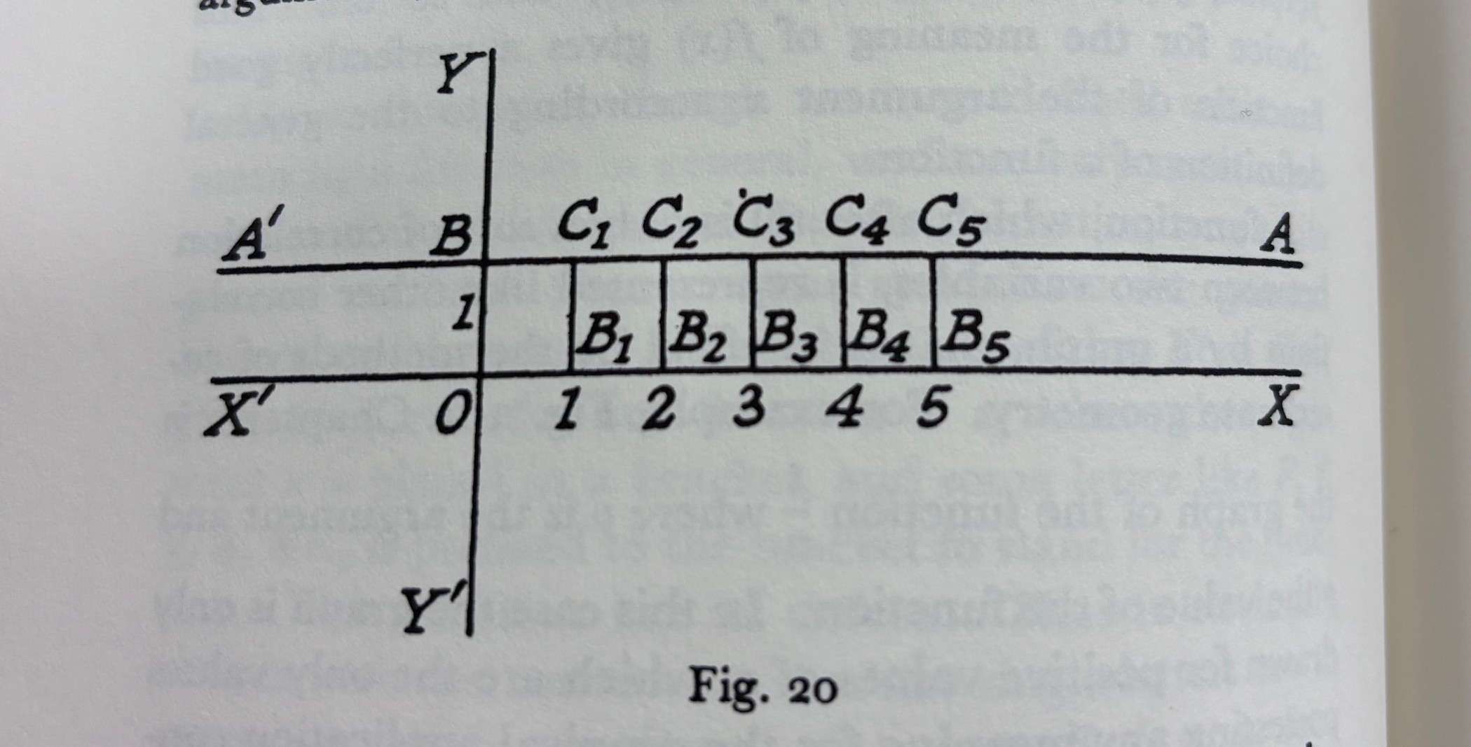
depicted in Chapter 2, if we only think of positive values of . But the function depicted in Fig.20 of
this chapter is discontinuous since at the values &c., of its argument, its
value gives sudden jumps.
Let us think of some examples of functions presented to us in nature,
so as to get into our heads the real bearing of continuity and
discontinuity. Consider a train in its journey along a railway line, say
from Euston Station, the terminus in London of the former London and
North-Western Railway. Along the line in order lie the stations of
Bletchley and Rugby. Let be the
number of hours which the train has been on its journey from Euston, and
be the number of miles passed
over. Then is a function of , i.e. is the variable value
corresponding to the variable argument . If we know the circumstances for the
train's run, we known as soon as
any special value of is given.
Now , miracles apart, we may confidently assume that is a continuous function of . It is impossible to allow for the
contingency that we can trace the train continuously from Euston to
Bletchley, and that then, without any intervening time, however short,
it should appear at Rugby. The idea is too fantastic to enter our
calculation: it contemplates possibilities not to be found outside at
the Arabian Nights; and even in those tales sheer discontinuity
of motion hardly enters into the imagination. they do not dare to tax
our credulity with anything more than very unusual speed. But unusual
speed is no contradiction to the great law of continuity of motion which
appears to hold in nature. Thus light moves at the rate of about 190,000
miles per second and comes to us from the sun in seven or night minutes;
but, in spite of this speed, its distance travelled is always a
continuous function of the time.
It is not quite so obvious to us that the velocity of a body is
invariably a continuous function of the time. Consider the train at any
time : it is moving withe some
definite velocity, say miles per
hour, where is zero when the
train is at rest in a station and is negative when the train is backing.
Now we readily allow that cannot
change its value suddenly for a big, heavy train. The train certainly
cannot be running at forty miles per hour from 11.45 a.m. up to noon,
and then suddenly, without any lapse of time, commence running at 50
miles per hour. We at once admit that the change of velocity will be a
gradual process. But how about sudden blows of adequate magnitude?
Suppose two trains collide; or, to take smaller objects, suppose a men
kicks a football. It certainly appears to our sense as though the
football began suddenly to move. Thus, in the case of velocity our
senses do not revolt at the idea of its being a discontinuous function
of the time, as they did at the idea of the train being instantaneously
transported from Bletchley to Rugby. As a matter of fact, if the laws of
motion, with their conception of mass, are true, there is no such thing
as discontinuous velocity in nature. Anything that appears to our senses
as discontinuous change of velocity must, according to them, be
considered to be a case of gradual change which is too quick to be
perceptible to us. It would be rash, however, to rush into the
generalization that no discontinuous functions are presented to us in
nature. A man who, trusting that the mean height of the land above
sea-leave between London and Paris was continuous function of the
distance from London, walked at night on Shakespeare's Cliff by Dover in
contemplation of the Milky Way, would be dead before he had had time to
rearrange his ideas as to the necessity of caution in scientific
conclusions.
It is very easy to find a discontinuous function, even if we confine
ourselves to the simplest of the algebraic formulae. For example, take
the function , which
we have already considered in the form , where was confined to positive values. But
now let have any value, positive
or negative. The graph of the function is exhibited in Fig.21. Suppose
to change continuously from a
large negative value through a numerically decreasing set of negative
values up to 0, and thence through the series of increasing positive
values. Accordingly, if a moving point, , represents on , starts at he extreme left of the axis
and successively moves
through &c. The
corresponding points on the function are &c. It is easy to
see that there is a point of discontinuity at , i.e. at the origin . For the value of the function on the
negative (left) side of the origin becomes endlessly great, but
negative, and the function reappears on the positive (right) side as
endlessly great but positive. Hence, however small we take the length
, there is a finite jump
between the values of the function at and . Indeed, this case has the
peculiarity that the smaller we take the length between and , so long as they enclose the origin,
the bigger is the jump in value of the function between them. This graph
brings out, what is also apparent in Fig.20 of this chapter, that for
many functions the discontinuities only occur at isolated points, so
that by restricting the values of the argument we obtain a continuous
function for these remaining values. Thus it is evident form Fig,21 that
in , if we keep to
positive value only and exclude the origin, we obtain a continuous
function. Similarly the same function, if we keep to negative values
only, excluding the origin, is continuous. Again the function which is
graphed in Fig.20 is continuous between and , and between and , and between and , and so on, always in each case
excluding the end points. It is , however, easy to find functions such
that their discontinuities occur at all points. For example, consider a
function , such that when
is any fractional number . This function is discontinuous
at all points.
Finally, we will look a little more closely at the definition of
continuity given above. We have said that a function is continuous when
its value only alters gradually for gradual alterations of the argument,
and is discontinuous when it can alter its value by sudden jumps. This
is exactly the sort of definition which satisfied our mathematical
forefathers and no longer satisfied modern mathematicians. It is worth
while to spend some time over it; for when we understand the modern
objections to it, we shall have gone a long way towards the
understanding of the spirit of modern mathematics. The whole difference
between the older and the newer mathematics lies in the fact that vague
half-metaphorical terms like 'gradually' are no longer tolerated in its
exact statements. Modern mathematics will only admit statements and
definitions and arguments which exclusively employ the few simple ideas
about number and magnitude and variables on which the science is
founded. Of two numbers one can be greater or less that the other; and
one can be such and such a multiple of the other; but there is no
relation of 'graduality' between two numbers, and hence the term in
inadmissible. Now this may seen at first sight to be great pedantry. To
this charge there are two answers. In the first place, during the first
half of the nineteenth century it was found by some great
mathematicians, especially Abel in Sweden, and Weierstrass in Germany,
that large parts of mathematics as enunciated in the old happy-go-lucky
manner were simply wrong. Macaulay in his essay on Bacon contrasts the
certainty of mathematics with the uncertainty of philosophy; and by way
of a rhetorical example he says.'There has been no reaction against
Taylor's theorem.' He could not have chosen a worse example. For,
without having made an examination of English text-books on mathematics
contemporary with the publication of the essay, the assumption is a
fairly safe one that Taylor's theorem was enunciated and proved wrongly
in every one of them. Accordingly, the anxious precision of modern
mathematics is necessary for accuracy. In the second place it is
necessary for research. It makes for clearness of thought, and thence
for boldness of thought and for fertility in trying new combinations of
ideas. When the initial statements are vague and slipshod, at every
subsequent state of thought common sense has to step in to limit
applications and to explain meanings. Now in creative thought common
sense in a bad master. Its sole criterion for judgement is that the new
ideas shall look like the old ones. In other words it can only act by
suppressing originality.
In working our way towards the precise definition of continuity (as
applied to functions) let us consider more closely the statement that
there is no relation of 'graduality' between numbers. It may be asked,
Cannot one number be only slightly greater than another number, or in
other words, cannot the difference between the two numbers be small? The
whole point is that in the abstract, apart form some arbitrarily assumed
application, there is no such thing as a great or small number. A
million miles is a small number of miles for an astronomer investigating
the fixed stars, but a million pounds is a large yearly income. Again,
one-quarter is a large faction of one's income to give away in charity,
but is a small fraction of it to retain for private use. Examples can be
accumulated indefinitely to show that great or small in any absolute
sense have no abstract application to numbers. We can say of two numbers
that one is greater or smaller than another, but not without
specification of particular circumstances that any one number is great
or small. Our task therefore is to define continuity without any mention
of 'small' or 'gradual' change in value of function.
In order to do this we will give names to some ideas, which will also
be useful when we come to consider limits and the differential
calculus.
为了做到这一点,我们将给一些概念命名,这些命名在我们考虑极限和微积分时也会很有用。
An 'interval' of value of the argument of a function is all the values lying between some
two values of the argument. For example, the interval between and consists of all the values which
can take lying between 1 and 2,
i.e. is consists of all the real numbers between 1 and 2. But the
bounding numbers of an interval need not be integers. An interval of
values of the argument a
number , when is a member of the interval. For
example, the interval between 1 and 2 contains and
so on.
A set of numbers approximates to a number within a , when the numerical
difference between and every
number of the set is less than .
Here is the 'standard of
approximation'. Thus the set of numbers approximates to the number 5
within the standard 4. In this case the standard 4 is not the smallest
which could have been chosen, the set also approximates to 5 within any
of the standards 3.1 or 3.01 or 3.001. Again, the numbers, 3.1, 3.141,
3.1415, 3.14159 approximate to 3.13102 within the standard 0.032, and
also within the smaller standard 0,03103.
These two ideas of an interval and of approximation to a number
within a standard are easy enough; their only difficulty is that they
look rather trivial. But when combined with the next idea, that of the
'neighbourhood' of a number, they form the foundation of modern
mathematical reasoning. What do we mean by saying that something is true
for a function in the
neighbourhood of the value of the
argument ? It is this fundamental
notion which we have now got to make precise.
The value of a function are
said to possess a characteristic in the 'neighbourhood of ' when some interval can be found which
(1) contains the number not as an
end-point and (2) is such that every value of the function for
arguments, other than , lying
within that interval possesses the characteristic. The value of the function for the argument
may or may not possess the
characteristic. Nothing is decided on this point by statements about
of a.
For example, suppose we take the particular function . Now of 2, the values of are less than 5. For we can find an
interval, e.g from 1 to 2.1, which (1) contains 2 not as an end-point,
and (2) is such that, for values of lying within it, is less than 5.
Now, combining the preceding ideas we know what is meant by saying
that the function approximates to within the . It means that some
interval can be found which (1) includes not as an end-point, and (2) is such
that all values of , where
lies in the interval and is not
, differ form by less than . For example, in the neighbourhood of
2, the function
approximates to 1,41425 within the standard 0.0001. This is true because
the square root of 1.99996164 is 1.4142 and the square root of
2.00024449 is 1.4143; hence for values of lying in the interval 1.99996164 to
2.00024449, which contains 2 not as an end-point, the values of the
function all line between
1.4142 and 1.4143, and they therefore all differ from 1.41425 by less
than 0.0001. In this case we can, if we like, fix a smaller standard of
approximation, namely 0.00051 or 0.000501. Again, to take another
example, in the neighbourhood of 2 the function approximates to 4 within the standard
0.5. For and , and thus the required
interval 1.9 to 2.1, containing 2 not as an end-point, has been found.
This example brings out the fact that statements about a function in the neighbourhood of a number
are distinct from statements
about the value of when . The production of an , throughout which the statement
is true, is required. Thus the mere fact that does not by itself justify us in
saying that in the of
2 the function is equal to 4.
This statement would be untrue, because no interval can be produced with
the required property. Also, the fact that does not by itself justify us in
saying that in the of
2 the function approximates to
4 within the standard 0.5; although as a matter of fact, the statement
has just been proved to be true.
If we understand the preceding ideas, we understand the foundations
of modern mathematics. We shall recur to analogous ideas in the chapter
on Series, and again in the chapter on the Differential Calculus.
Meanwhile, we are now prepared to define 'continuous functions'. A
function is 'continuous' at a
value of its argument, when in
the neighbourhood of its values
approximate to f(a) (i.e. to its value at ) within standard of approximation.
This means that, whatever standard be chosen, in the neighbourhood of
approximates to within the standard . For example, is continues at the values 2 of its
argument, , because however be chosen we can always find an
interval, which (1) contains 2 not as an end-point, and (2) is such that
the values of for arguments
lying within it approximate to 4 (i.e. ) within the standard . Thus, suppose we choose the standard
0.1; now , and
, and both these
numbers differ from 4 by less than 0.1. Hence, within the interval 1.999
to 2.01 the values of
approximate to 4 within the standard 0.1. Similarly an interval can be
produced for any other standard which we like to try.
Take the example of the railway train. Its velocity is continuous as
it passes the signal box, if whatever velocity you like to assign (say
one-millionth of a mile per hour) an interval of time can be found
extending before and after the instant of passing, such that at all
instants within it the train's velocity differs from that with which the
train passed the box by less than one-millionth of a mile per hour; and
the same is true whatever other velocity be mentioned in the place of
one-millionth of per hour.